Streamlining Adobe Audience Manager with Snowflake

[#1]

Authors: Navin Chaganti and Jenny Medeiros

The following is a practical overview of why we transitioned from Amazon Redshift to Snowflake to streamline Adobe Audience Manager within Adobe Experience Platform.

Marketers use Adobe Audience Manager to seamlessly collect and merge data from multiple sources, build meaningful audience segments, and deliver customer-focused experiences in real-time.

Behind the scenes of this powerful data management platform, trillions of batch and real-time data are processed every single day. Back in 2016, we selected Amazon Redshift to handle this hefty task. But, with the exploding demand for data-driven insight, this solution began to stumble in the race to provide the scale, speed, and flexibility needed to serve our growing customer base. Heavy workloads often bled into the weekends, resizing clusters was a recipe for downtime, and there was virtually no time left for maintenance.

To remedy these setbacks, we moved from Amazon Redshift to Snowflake – a zero-maintenance cloud data warehouse that grants efficient query processing, flexible workload management, and seamless scaling.

In this post, we compare Amazon Redshift to Snowflake in the context of the specific use case: trait-to-trait overlap. We also describe our current workflow using Snowflake's innovative solution.

Adobe Audience Manager and overlap reports

Today, marketers have enormous amounts of siloed datasets and audience data assets – such as first, second, and third party data. They define this information in Adobe Audience Manager as signals, traits, and segments.

• Signals represent either user interaction or user activity on a customers' online property (e.g. clicking on an Adobe Photoshop ad).
• Traits are combinations of one or more signals that qualify a user for an audience segment (e.g. "Adobe visitor", "Photoshop fan").
• Segments are combinations of one or more traits (e.g. "Adobe visitor" + "Photoshop fan" = Adobe Creative Cloud audience).

Adobe Audience Manager ingests billions of real-time and batch events and activates trillions of segments and traits every day to create meaningful audience segments. This allows marketers to target the right audience with the most relevant content across multiple digital channels. But, it also results in an extremely heavy and expensive compute.

One operation that requires such resource-intensive jobs is called overlap, which determines the common users between multiple segments and multiple traits. For example, consider a company with two segments: one with 2,000 Star Wars fans and another with 1,000 Star Trek fans. If 500 users belong to both segments, that is an overlap.

Figure 1: Venn diagram illustrating an overlap.

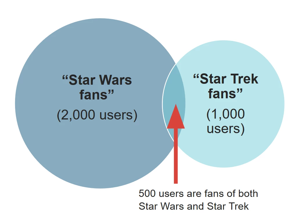
Once Adobe Audience Manager generates an overlap report, advertisers can choose to either optimize their media spend and target only those 500 unique users with ads for space adventure products or cast a wider net by targeting more users.

For example, imagine a toy company has $100 to target 100 Star Wars and Star Trek fans with digital ads. If it takes $1 to target one user, then the company would spend all $100 on its audience.

With an overlap report in hand, however, the company would know that 50 of those 100 people are fans of both Star Trek and Star Wars. This means that if they spent $100 on both segments, they would only reach 50 unique users. Instead, the company can spend only $50 on those 50 fans who have a higher chance of clicking on the ad. They can then use the rest of the money to reach more users in other potential segments, such as Guardians of the Galaxy fans.

To illustrate the challenge of calculating the overlap report with Redshift versus Snowflake, we will consider a particular kind of overlap: trait-to-trait overlap.

Trait-to-trait overlap: Redshift Vs. Snowflake

A trait-to-trait overlap is the percentage of unique users shared between all the customer's first and third-party traits. A first-party trait is, for example, when a user clicks on Adobe Photoshop's webpage. A third-party trait is obtained from vendors and data aggregators, drawing extra information like "man working in tech under 30 years old."

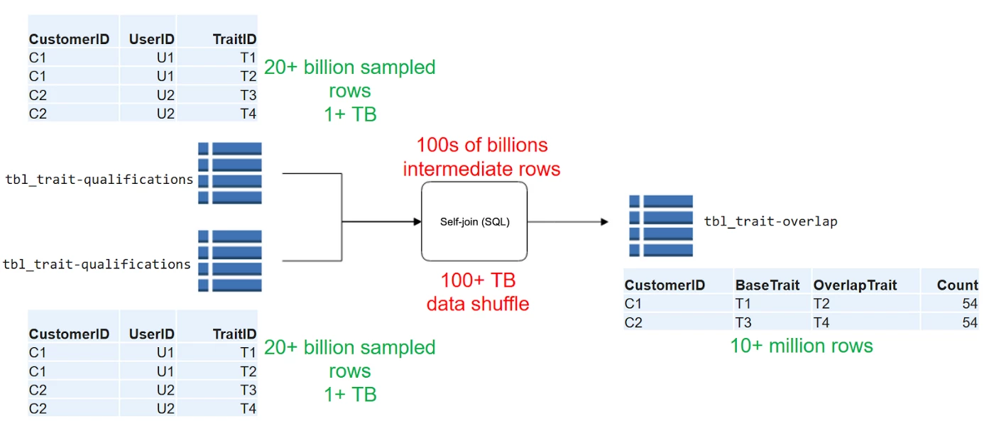
To calculate a trait-to-trait overlap report, Adobe Audience Manager performs a self-join – a cartesian product to compute pairs of traits with common user ID's in the last 30 days. This is done for every customer.

In 2016, Adobe Audience Manager had around 900 customers, who set more than 1.5 million first-party traits and 150,000 third-party traits. This totaled to over 50 billion daily trait qualifications (i.e. user interactions).

To put it into perspective, if performing a self-join on three traits creates six combinations, imagine the sheer number of combinations from 50 billion traits.

With this scale of data in mind, we will now describe how Amazon Redshift handled this complex use case, followed by Snowflake's approach and how it fits into our current workflow.

Amazon Redshift

Back in 2016, we used Amazon Redshift to run our overlap query. The trait-qualification table for Amazon redshift at the time had around three trillion rows with a retention of 60 days and 60+ TB of data. To optimize query performance for overlap processing, we statistically sampled the data down to 20 billion rows. But with Amazon Redshift, each self-join generated billions of intermediate rows and hundreds of TBs of data. (See figure below.)

Figure 2: Overlap processing workflow in Amazon Redshift.

To distribute the data on the Amazon Redshift cluster, we used the user_id as the DISTKEY. In the current implementation, however, our cluster was split in two: an 18-node cluster that processed all our heavy computation queries, and a two-node cluster that powered our Tableau reports.

Figure 3: Overlap reporting stack with Amazon Redshift.

In total, our cluster had a memory of 2.1 TB, 288 cores, and 288 TB of storage. With this amount of memory, shuffling data between the cores was a painfully slow operation. Furthermore, each single-threaded query ran concurrently and blocked any other jobs from running, which inevitably caused major blockages as the number of jobs increased.

As a consequence, our query runtime was exceedingly extensive and predicted to slow down even further as our database grew. See the graph below.

Figure 4: Graph showing hours spent on overlap processing in Amazon Redshift.

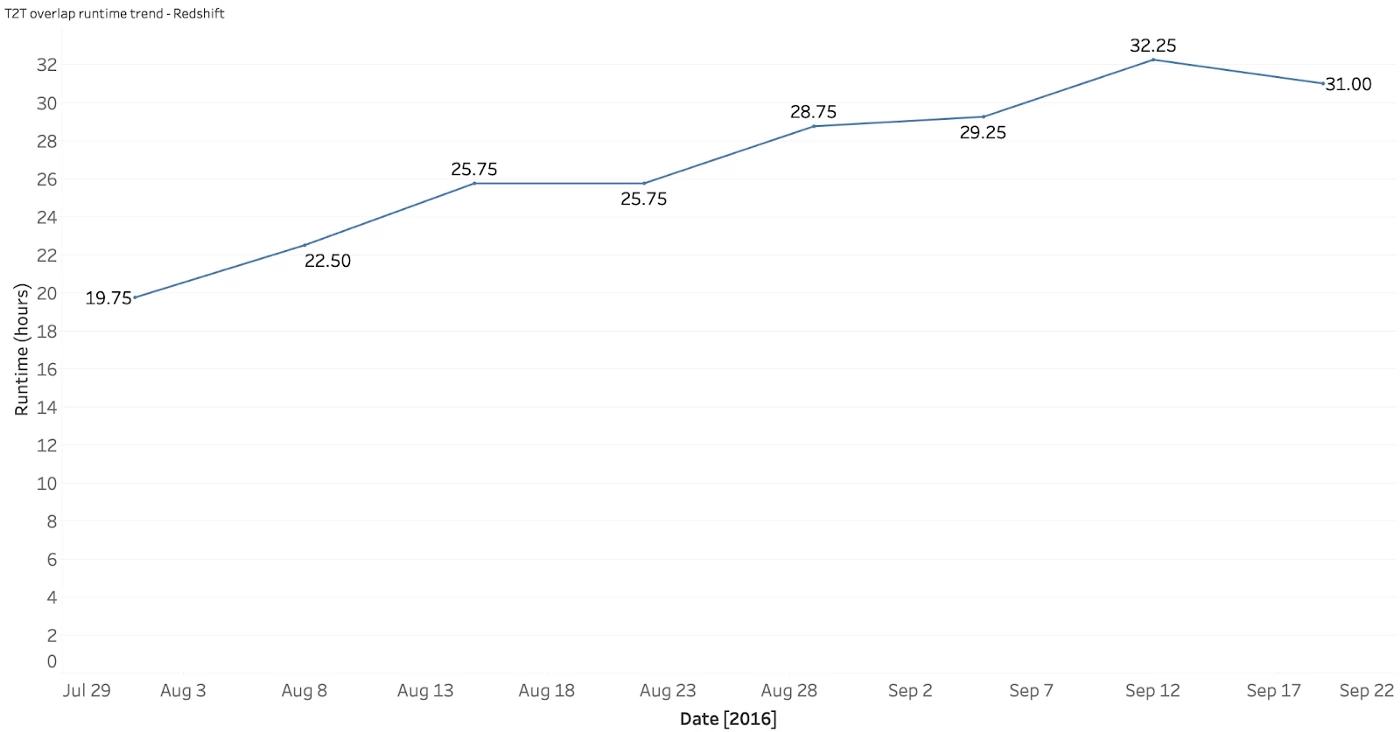
As shown in the graph, the query time for overlap reports on the 18-node Amazon Redshift cluster steadily increased from 19.75 hours in July to 31 hours in September. To add insult to injury, if a failure occurred after 30 hours we had to restart the query and wait almost two additional days of runtime. By then, the customer's SLA had likely expired.

Snowflake

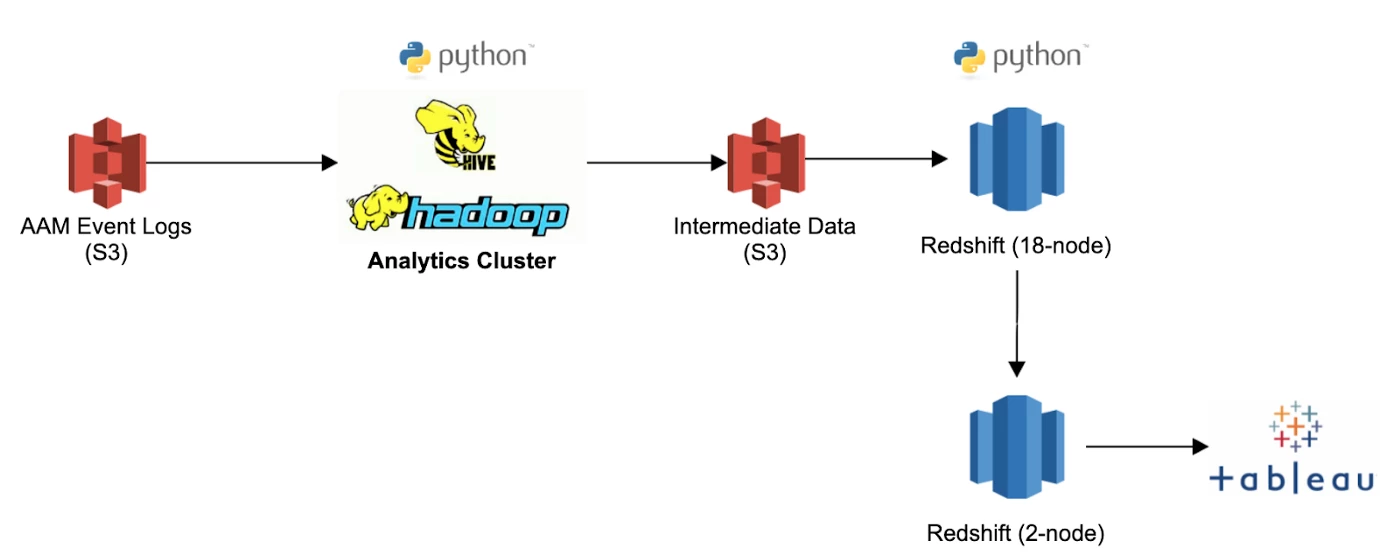
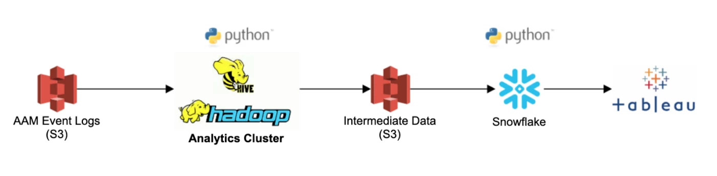
Three years later, we decided to implement Snowflake and re-architect our entire reporting workflow (see image below). This reporting workflow is not only used for overlaps, but for all our reporting workloads.

Figure 5: Snowflake reporting workflow.

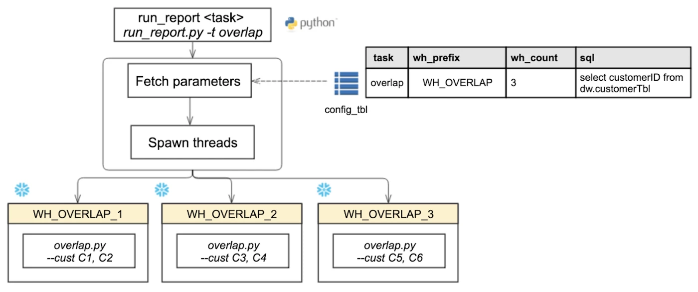
In this new workflow, we built a new wrapper script called run_report and configured it so we could scale the cluster simply by entering the number of warehouses we want to spin. The script then spins the warehouses and distributes the data across them.

To achieve this, the configuration table shown in the image above is comprised of the following:

• Task: Name of the task.
• Wh_prefix: Prefix to be attached to the upcoming warehouse.
• Wh_count: Number of warehouses launched to compute the task.
• SQL: Returns the number of clients to be computed.

In keeping with the table shown, consider the following example: if the script launches three warehouses and there are six clients coming from the SQL, the script distributes the clients C1 – C6 in a round-robin fashion to each warehouse. This ensures that both the data and the load of the compute are spread equally among the warehouses.

As such, the clients in this scenario would be dealt as follows:

• C1, C2 to wh_overlap_1
• C3, C4 to wh_overlap_2
• C5, C6 to wh_overlap_3

This renovated workflow also bred a new overlap processing architecture, as shown in the image below.

Figure 6: Overlap processing workflow in Snowflake.

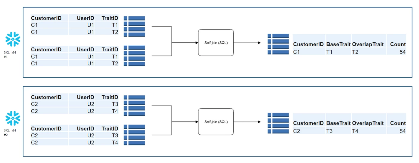
Instead of running a single-threaded self-join on 20 billion rows, in Snowflake the data is split between two warehouses where both queries are run in parallel. This more than halves the amount of intermediate data and noticeably improves query performance. As a result, query times fell from 31 hours to only 8 hours.

Figure 7: Graph showing hours spent on overlap processing in Snowflake.

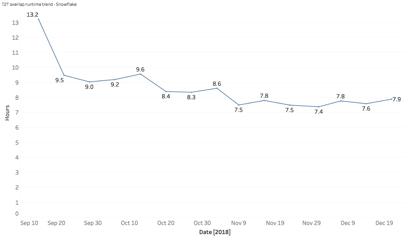
As shown in the graph above, execution time has drastically reduced over time. Due to this vast improvement, we replaced Amazon Redshift entirely in our reporting stack.

Figure 8: Current reporting stack using Snowflake.

As a result, our current trait-qualification table has gone from 60 days of retention, 60+ TB of data, and 3 trillion rows to just 45 days of retention, 400 TB of data, and almost 30 trillion rows. While we have effectively scaled 10x in just three years, all we need to do is make a small configuration change to handle it. No code changes, no downtime, and no weekend work shifts.

Key takeaways after transitioning to Snowflake

When we began three years ago, we were spending eight hours resizing clusters, running extensive queries concurrently, and struggling to find time for much-needed maintenance.

After moving to Snowflake, we can instantly scale a cluster in a few clicks, easily configure multi-threaded jobs to run in parallel (and independently), and have no need to maintain the system ourselves. Not only has this saved on costs and returned our weekends, but it also freed our team to focus on innovating new features for Adobe Audience Manager.

By implementing Snowflake, we also highlighted the importance of configurable warehouse settings to accommodate spiky workloads. We also noted the need for multi-threading ETL jobs operating on TB-scale datasets. Furthermore, such large datasets must ensure automated data retention to prevent the escalation of storage costs.

Ultimately, Snowflake has smoothed and polished the reporting workflow so we can continue providing customers of Adobe Audience Manager with the powerful, real-time insights they need when they need it.

Follow the Adobe Experience Platform Community Blog for more developer stories and resources, and check out Adobe Developers on Twitter for the latest news and developer products. Sign up here for future Adobe Experience Platform Meetups.

Originally published: Dec 5, 2019