Selecting the Best Attribution Model Using Adobe's Attribution Lift Measure

[#1]

Authors: Jim Snyder, Arava Sai Kumar, and Kimberly Leung (@kimberlyl468851)

This post explores how we select the best attribution model in a data-driven way using Adobe’s Attribution Lift Measure (ALM). This approach avoids the need for expensive experiments or simulations to evaluate the effectiveness of both traditional rules-based and sophisticated machine-learning-based attribution models.

Marketing teams frequently use attributional models to understand what marketing investments like campaigns and advertisements deserve credit for conversions, such as purchasing a product. These models work by assigning a fraction of credit to each advertisement (or marketing touchpoint) along their consumers’ journeys. With this information, marketers can better design future campaigns, bid efficiently on advertising space, and optimize their marketing spend to maximize return on investment. There is one caveat here. The ability to do this effectively depends significantly on the marketer’s choice of attribution model.

Types of Attribution Models

Traditionally, marketing teams have relied on a variety of rules-based heuristics for assigning credit to marketing channels. More recently, to more accurately assign credit, marketers and data scientists have developed algorithmic models, which use more sophisticated data-driven and machine learning techniques to determine how credit is allocated to marketing and advertising touchpoints.

Some of the most common models are:

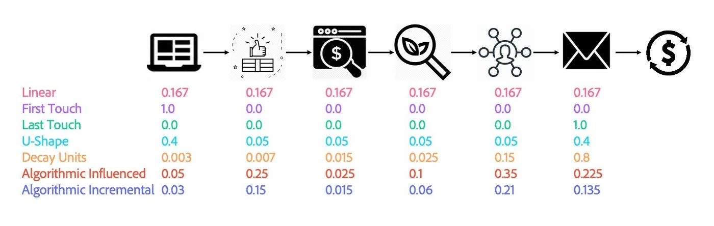
• Linear: All touchpoints along the consumer journey are assigned equal credit for the conversion event.
• First-Touch: The first touchpoint on the consumer journey is assigned 100% of the credit for the conversion event.
• Last-Touch: The last touchpoint on the consumer journey is assigned 100% of the credit for the conversion event.
• U-Shape: The first and last touchpoints are assigned an equal amount of credit for the conversion event that is more than the other touchpoints in the middle of the consumer journey. The remaining credit is then distributed evenly amongst the other touchpoints.
• Decay Units (Time Decay): Credit is assigned with respect to time. Credit is assigned to all the touchpoints along the consumer journey, with the amount of credit exponentially decaying as it is further back in time from the conversion event.
• Algorithmic Influenced (Fractional): 100% of the conversion credit is algorithmically distributed amongst all the touchpoints along the consumer journey.
• Algorithmic Incremental: The proportion of the credit due to marketing is algorithmically distributed amongst the touchpoints along the consumer journey. Unlike algorithmic influenced, this may not sum to 100% because marketing may only be partially responsible for the conversion.

Figure 1: An example illustrating how different attribution models work when applied to a sample conversion path.

Challenges with Current Model Selection Tactics

For marketers, it is difficult to determine which model, or combination of models, is best. The choice of model(s) often comes down to the subjective and unmeasurable preferences of their teams and stakeholders.

A major reason why attribution model selection is quite subjective and an objective evaluation is very difficult is due to the fact that evaluation methods that are widely used in other contexts are typically not practical, extremely expensive to run, or have many limitations. Here are some examples of common evaluation methods: experiments, simulations, and model fit metrics.

Experiments

A/B testing is an experiment method commonly used by technology companies to determine whether a product change is beneficial to their platform. An A/B test involves randomly breaking similar users into two different groups–control and test groups.

The users in the control group use the current version of the product, and those in the test group are exposed to the change. Then, experimenters monitor these two groups over time to see if there is a meaningful difference in a key success metric, such as average usage time. Importantly, these two groups must be evaluated at the same time to control for confounding factors, such as a recession.

A/B tests, if designed properly, are very rigorous and establish a causal relationship between the change and key success metrics. However, they have some nontrivial drawbacks.

• They are expensive and time-consuming to set up, often taking weeks or months to collect data and evaluate. For example, the phase III clinical trials, which are akin to A/B tests, of the various COVID-19 vaccines took several months to run.
• They need to be designed carefully to prevent confounding factors from introducing misleading results. As an example, a company may decide to make their control group North America and their test group the UK. The problem here is that these two groups are dissimilar in nontrivial ways. For example, a geopolitical event, such as Brexit, may have a large impact on consumer behavior in the UK. However, the impact of Brexit is likely much smaller in North America. Any changes observed may be a result of this event, as opposed to the experiment change.
• There are a wide variety of other common mistakes made, which have been summarized in other places a....

As a result, many companies do not have the budget or are otherwise unwilling to run these types of experiments. Despite this, it should be possible to run an A/B test to determine the best attribution model, and this and other similar experiments are ultimately the gold standard in terms of proof and establishing causality.

Simulations

Besides experiments, simulations can be used to prove that a model is better than other models. Simulations work by building a model that uses controllable inputs, such as marketing spend on different advertisements, to predict an output, such as ROI. If a model can predict ROI well, given an input, then it is possible to simulate adjustments to the input and see the impact on the output.

The advantage of simulations is that, once the right simulation is discovered, it is much less expensive and time-consuming than an experiment. Typically, it only takes several days to weeks to run a simulation, instead of weeks to months to run an experiment.

However, the challenge is that it is very difficult to discover an accurate simulation. It often requires significant time investment upfront from a team of data scientists to research and identify an accurate simulation. Since simulations are often built using deep learning, the computational requirements for these simulations are often high. Arguably the most significant issue with simulations is that there will be natural questions about their trustworthiness. One such argument is that marketing relationships are complex and dynamic: an accurate simulation for today may not generalize well for the future.

Model Fit Metrics

When discussing models, it is not uncommon to hear that one model is better than another because it has a higher R² or AUC, which are examples of model fit metrics. Model fit metrics are tools used to determine how well a model explains the data by measuring prediction accuracy and errors.

In fact, model fit metrics are very useful to help determine when one model is better than another, but they have some limitations. First, these metrics can’t be produced for rules-based heuristics, meaning they can’t help prove that a machine-learning-based model is better than a rules-based model. There are some exceptions to this statement, but they do not apply to attribution models. While many data scientists may scoff at the notion that a rules-based model could be better than a machine learning-based model, it is very much possible for this to be the case if the model is not well developed. Furthermore, business stakeholders often challenge and demand proof that the algorithmic models are superior to the existing models that they have been using.

Beyond this issue, model fit metrics only evaluate how well the model does on what it is trained to do (e.g. predicting whether a user converts or not). However, any additional transformations to the results after training are not evaluated by these methods. This is directly relevant to attribution. In Adobe’s Attribution AI product, there are two different algorithmic scores, incremental and influenced, and both are produced by the same model. Influenced scores for each conversion must sum to 1.0, which is typical of most rules-based methods, and are scaled accordingly. Incremental scores may sum to something less than or equal to 1.0. This is because the incremental scores are the marginal increase in the probability of converting, and the conversion probability is typically less than 1.0. In contrast, the influenced scores are the fraction of marketing credit belonging to each touchpoint.

The output from these two approaches can be nontrivially different. As such, one of these models could be better than the other, despite having the same model fit metrics. Although existing model fit measurement methods cannot compare attribution models effectively, they have a big advantage over simulations and experiments. They are very fast to compute, taking seconds to hours. As a result, developing a novel model fit measurement method for attribution that applies both to rules-based and algorithmic models is highly desirable.

Attribution Approach

Consumer journeys that end in a conversion look different than ones that don’t because consumers exposed to a more effective marketing strategy are more likely to convert. Because of this, certain combinations of marketing touchpoints are more likely to appear on journeys that end in a conversion versus ones that don’t. Intuitively, a good attribution model should emphasize the touchpoints more commonly appearing on conversion paths by assigning more credit to them.

To illustrate this point, consider the following example, which is summarized pictorially in Figure 2. The arrow points to boxes indicating the degree of evidence that the advertisement contributed to the conversion. The next arrow shows how the ads should impact the model lift measure in good models.

• Say there are 100 potential customers. 50 of them saw a particular advertisement and bought the product, and the 50 remaining people neither saw the advertisement nor bought the product. Most people would agree that this is pretty strong evidence that the ad was effective and deserves some credit for the purchases.
• In another case, say 50 people converted and saw the ad, and 50 did not convert but saw the ad. While it is certainly possible that some of the people converted because they saw the ad, most people would agree that there is a much less compelling reason to believe the ad deserves a lot of credit.
• As a rather absurd case, 50 people converted, but only 1 person saw the ad, and 50 people saw the ad and did not convert. Most people would agree that this ad was not effective and likely does not even deserve much credit for the one person that saw it and converted.

Figure 2: Provides a series of examples where an advertisement may have contributed to conversions.

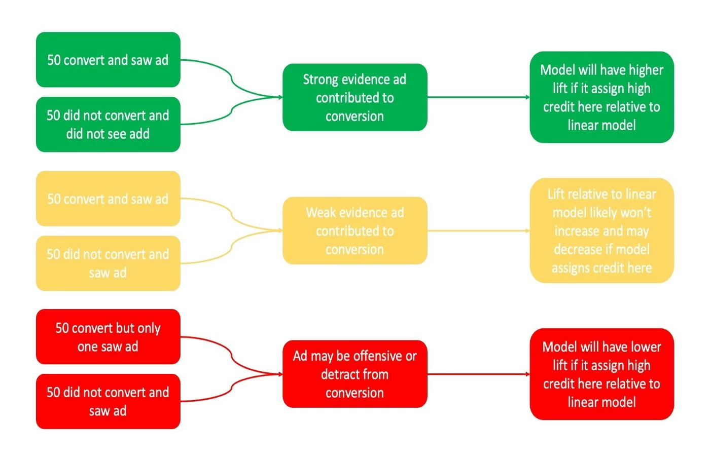
Although this example ignores many of the complexities in advertising (people don’t all respond the same way to the same ad), the critical point is that an advertisement deserves more credit as the difference between consumers’ behavior exposed and not exposed increases. Fortunately, the extent to which different attribution models assign credit in this way can be measured and compared.

Attribution Model Lift Measure

The Attribution Model Lift Measure (ALM) (US Patent Application Number: 17/146,655) is a custom measure of model fit tool designed to compare both rules-based and algorithmic attribution scores, including any score transformation done to the raw model output. Since this article is not meant to be technical, the details of how ALM is computed are not discussed here. At a high level, we only need two things to compute ALM.

1. The input data to generate paths that both end with and without conversions, where a path is a series of touchpoints. These are called positive and negative paths respectively.
2. Scored data using a variety of attribution models.

This is information that all attribution models either use or produce. To evaluate each model, we want to be able to evaluate how the attribution scores make the positive path data look more dissimilar to the negative paths because this is evidence that they are correctly assigning credit to touchpoints that tend to be more common on positive paths. To accomplish this, we do the following.

1. Convert the different data sources into probability distributions.
2. Measure the divergence between each attribution model distribution and one or more raw data distributions
3. Use the divergence to compute the lift to a baseline model, which is one model chosen to compare each of the other models.

The positive and negative distributions measure the prevalence of certain touchpoints on conversion and conversion-less paths, and a third distribution that we call the reference distribution measures the deviation between positive and negative paths. The attribution model distributions measure the magnitude of credit that different models give different touchpoints and can be thought of as the positive path distribution that is weighted by the attribution scores.

This process is illustrated in Figure 3 below. Although probability distributions are used to make comparing the different data sources easier, they just represent how common different touchpoints (in this case at certain time horizons from the conversion) are on different paths, where the score path also reflects how important the touchpoint is considered by the model. As you can see, the attribution model should make the positive paths look more dissimilar to the negative paths, resulting in the divergence increasing relative to the negative path distribution.

Figure 3: An example of probability distributions for the positive, negative, and score (attribution model) paths.

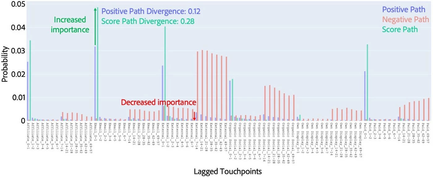
We convert the input data and scores into probability distributions primarily because these are required to compute statistical divergence, which is a rigorous way to evaluate the similarity between the positive and negative paths and the attribution model scores. We compute the divergence between the attribution model distributions and both the negative and reference distribution.

The first of these two divergences measure the extent to which attribution models credits touchpoints that are infrequently on negative paths, and the second measures the extent to which the attribution models reflect the deviation between positive and negative paths.

The final ALM indicates to what extent an attribution model better emphasizes the difference between positive and negative paths and concentrates credit on touchpoints that infrequently appear on negative paths when compared to a baseline model. The baseline model can be any model because the rank ordering of the models by lift will not change with different baselines.

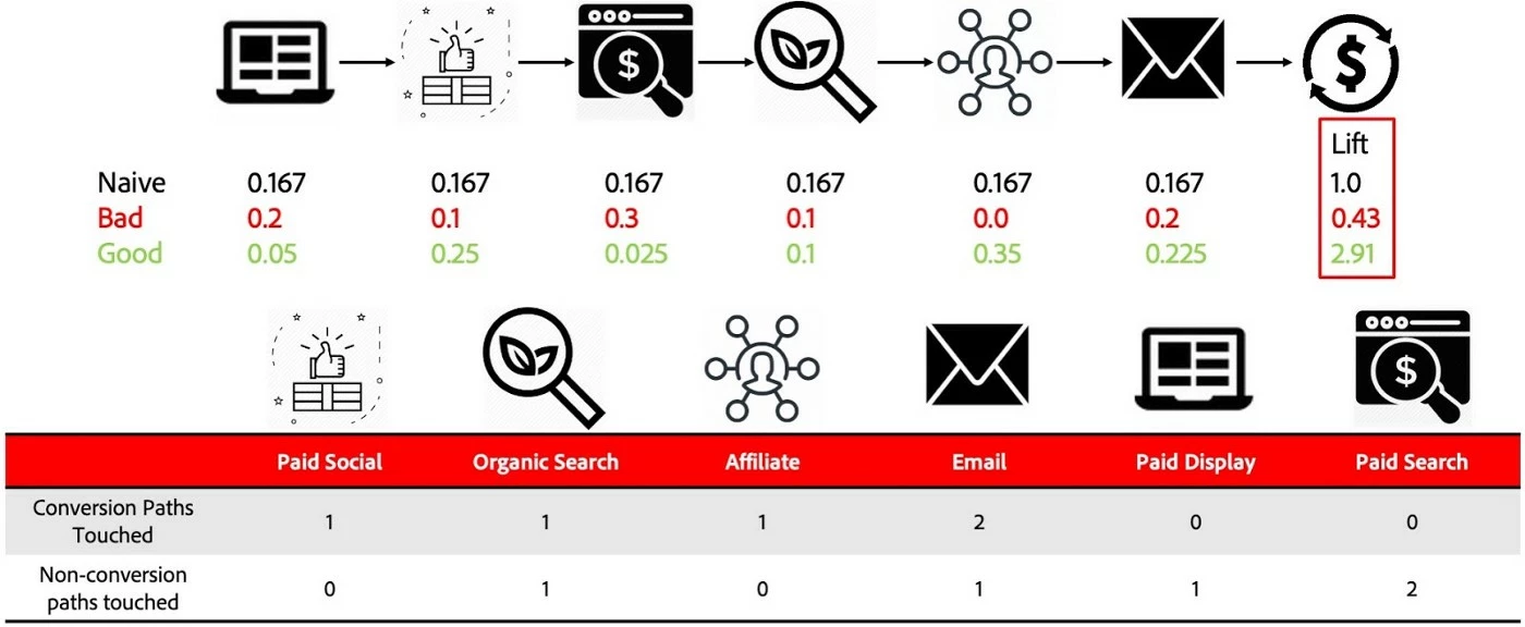
We typically use either a simple model (e.g. a linear model) or the model currently being used by a business. This is demonstrated in Figure 4, which compares a baseline linear model, bad attribution model, and good attribution model. The corresponding ALM is also shown. The table below shows the number of each touchpoint on conversion and conversion-less paths, indicating why the above scores are bad or good. The best model assigns high credit to touchpoints that frequently appear on negative paths, and the bad model does the opposite.

Figure 4: Shows an attribution path with three different scoring schemes.

Interpretation

The reason that we produce ALM is that it has a significant value in terms of interpretation. When comparing two models, one can think of the model lift as the percent improvement of one versus the other. For example, a lift of 1.2 means that the model is 20% better than the baseline at concentrating credit on touchpoints that frequently appear on conversion paths and infrequently appear on conversion-less paths and/or simply rarely appear on conversion-less paths.

In contrast, a lift of 0.8 means the model is 20% worse than the baseline at the same thing. It is possible to compare more than two models as well, and the higher the lift means the better each model is relative to the baseline. Beyond this, ALM also makes it possible to evaluate models across multiple applications.

Each model may be more or less accurate depending on how large the difference is between conversion and conversion-less paths, so the measure of model fit methods, like AUC, as well as the divergence calculations that comprise ALM, may vary accordingly. However, ALM only reflects how well one model performs relative to another and can be compared across applications.

Figure 5: A sample visualization of ALM, where several models are compared.

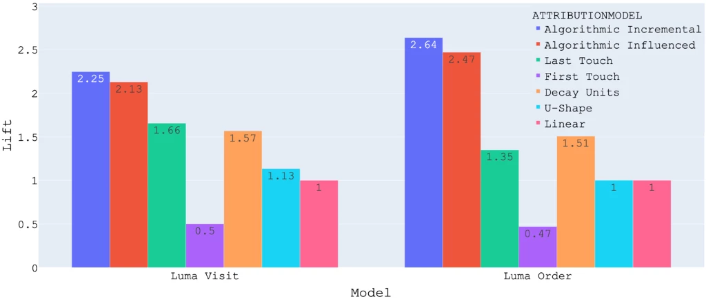
Since ALM measures the extent to which different models effectively assign credit to touchpoints that frequently appear on conversion paths and infrequently appear on conversion-less paths, models with higher ALMs are more accurately assigning credit to more effective touchpoints. By extension, we would expect the use of the model with the highest ALM to be correlated with higher ROI for marketing spend, though this cannot be guaranteed if the data quality isn’t good or the data isn’t reasonably stable.

Additionally, the ROI lift from using a particular model may not be the same as ALM, meaning a 50% ALM may not result in a 50% ROI lift. That being said, this is a rigorous way of determining a rank-ordered list of which models are likely to have the best impact on ROI. If nothing else, ALM should be used to select which models a marketing team will run experiments, as there is no practical way to test every possible model. However, if there are no plans to run A/B tests, it would be very reasonable to use the model with the highest ALM outright.

Closing Thoughts

Although many organizations want to optimize their marketing strategies, they are reluctant to do so–why fix something that is not broken when the cost to benefit analysis cannot be easily done?

Intuitively, we know that adopting an optimal attribution strategy will help optimize the holistic marketing strategies by better identifying the true value and efficiencies of marketing efforts against goals and telling that story to stakeholders. The conundrum is that it is extremely hard to select the optimal attribution model.

Adobe’s Attribution Model Lift Measure (ALM) is a cost-effective and straightforward tool that can help marketers to identify the best model and, more importantly, quantify why. Especially in the ever-accelerating digital transformation of consumer behavior and fragmentation of marketing channels, organizations cannot afford to move slowly and hesitate to adopt new strategies. We encourage marketers to embrace this new measure and quickly adopt an optimal attribution model to help them make smarter and faster decisions to optimize their strategies and maximize marketing ROI.

Adobe is making strides within the marketing and measurement space, especially by harnessing advanced AI and ML technologies to solve complex marketing problems. Please continue to follow this blog to learn more about the research and upcoming innovations.

Follow the Adobe Experience Platform Community Blog for more developer stories and resources, and check out Adobe Developers on Twitter for the latest news and developer products. Sign up here for future Adobe Experience Platform Meetups.

References

1. Attribution AI Overview
2. Ten common A/B testing pitfalls and how to avoid them
3. Probability Distribution Overview
4. Statistical Divergence Description

Originally published: Apr 1, 2021