Taking Query Optimizations to the Next Level with Iceberg

[#1]

Authors: Gautam P. Kowshik and Xabriel J. Collazo Mojica

This blog is the third post of a series on Apache Iceberg at Adobe. In the first blog we gave an overview of the Adobe Experience Platform architecture. We showed how data flows through the Adobe Experience Platform, how the data’s schema is laid out, and also some of the unique challenges that it poses. We also discussed the basics of Apache Iceberg and what makes it a viable solution for our platform. Iceberg today is our de-facto data format for all datasets in our data lake.

We covered issues with ingestion throughput in the previous blog in this series. We will now focus on achieving read performance using Apache Iceberg and compare how Iceberg performed in the initial prototype vs. how it does today and walk through the optimizations we did to make it work for AEP.

Here are some of the challenges we faced, from a read perspective, before Iceberg:

• Consistency Between Data & Metadata: We had all our metadata in a separate store from our data lake as most big data systems do. This made it hard to do data restatement. Restating thousands of files in a transactional way was difficult and error-prone. Readers were often left in a potentially inconsistent state due to data being compacted or archived aggressively.
• Metadata Scalability: Our largest tables would easily get bloated with metadata causing query planning to be cumbersome and hard to scale. Task effort planning took many trips to the metadata store and data lake. Listing files on data lake involve a recursive listing of hierarchical directories that took hours for some datasets that had years of historical data.
• Inefficient Read Access: For secondary use cases, we often ended up having to scan more data than necessary. Partition pruning only got us very coarse-grained split plans. As an example, complying with GDPR requires finding files that match data for a set of users. This required a table with a time-series partitioning scheme that was a full table scan even if the actual set of matching files was relatively small.

Read Access in Adobe Experience Platform

Adobe Experience Platform keeps petabytes of ingested data in the Microsoft Azure Data Lake Store (ADLS). Our users use a variety of tools to get their work done. Their tools range from third-party BI tools and Adobe products. Because of their variety of tools, our users need to access data in various ways.

Additionally, our users run thousands of queries on tens of thousands of datasets using SQL, REST APIs and Apache Spark code in Java, Scala, Python and R. The illustration below represents how most clients access data from our data lake using Spark compute.

Figure 1: Client Access to Adobe Experience Platform data lake

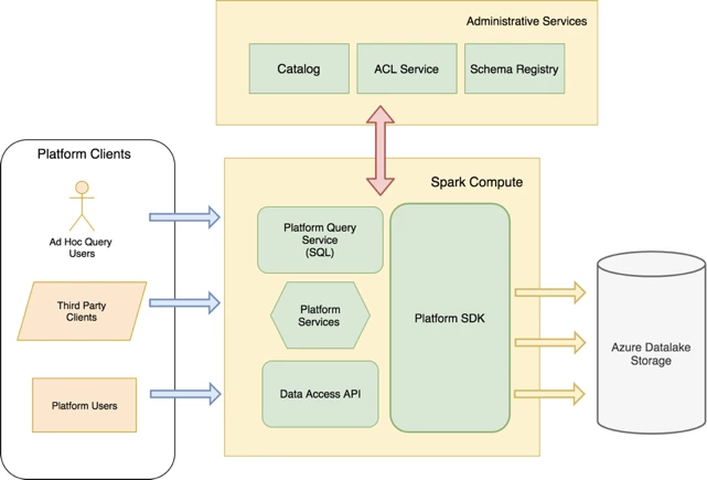
Our platform services access datasets on the data lake without being exposed to the internals of Iceberg. All read access patterns are abstracted away behind a Platform SDK. All clients in the data platform integrate with this SDK which provides a Spark Data Source that clients can use to read data from the data lake. This is the standard read abstraction for all batch-oriented systems accessing the data via Spark.

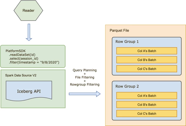
Underneath the SDK is the Iceberg Data Source that translates the API into Iceberg operations. This allowed us to switch between data formats (Parquet or Iceberg) with minimal impact to clients. The picture below illustrates readers accessing Iceberg data format. Query planning and filtering are pushed down by Platform SDK down to Iceberg via Spark Data Source API, Iceberg then uses Parquet file format statistics to skip files and Parquet row-groups.

Figure 2: Reading with Iceberg Over Parquet

Iceberg for Reading

Iceberg is a library that offers a convenient data format to collect and manage metadata about data transactions. Iceberg’s APIs make it possible for users to scale metadata operations using big-data compute frameworks like Spark by treating metadata like big-data. At its core, Iceberg can either work in a single process or can be scaled to multiple processes using big-data processing access patterns.

Iceberg APIs control all data and metadata access, no external writers can write data to an iceberg dataset. This way it ensures full control on reading and can provide reader isolation by keeping an immutable view of table state. Using snapshot isolation readers always have a consistent view of the data. In our earlier blog about Iceberg at Adobe we described how Iceberg’s metadata is laid out.

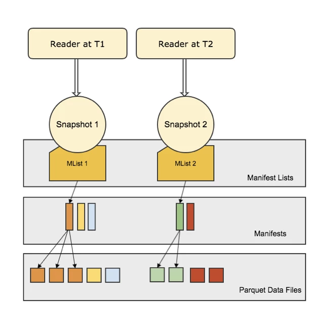
A reader always reads from a snapshot of the dataset and at any given moment a snapshot has the entire view of the dataset. Underneath the snapshot is a manifest-list which is an index on manifest metadata files. Manifests are Avro files that contain file-level metadata and statistics. The diagram below provides a logical view of how readers interact with Iceberg metadata.

Figure 3: Reader Snapshot Isolation

Query Planning

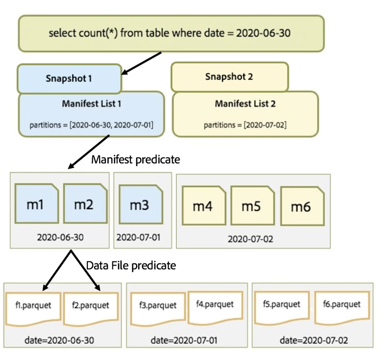
Before Iceberg, simple queries in our query engine took hours to finish file listing before kicking off the Compute job to do the actual work on the query. To even realize what work needs to be done, the query engine needs to know how many files we want to process. For most of our queries, the query is just trying to process a relatively small portion of data from a large table with potentially millions of files. Iceberg design allows for query planning on such queries to be done on a single process and in O(1) RPC calls to the file system.

Iceberg knows where the data lives, how the files are laid out, how the partitions are spread (agnostic of how deeply nested the partition scheme is). Furthermore, table metadata files themselves can get very large, and scanning all metadata for certain queries (e.g. full table scans for user data filtering for GDPR) cannot be avoided. For such cases, the file pruning and filtering can be delegated (this is upcoming work discussed here) to a distributed compute job.

Iceberg treats metadata like data by keeping it in a split-able format viz. Avro and hence can partition its manifests into physical partitions based on the partition specification. Iceberg keeps two levels of metadata: manifest-list and manifest files. This two-level hierarchy is done so that iceberg can build an index on its own metadata. This layout allows clients to keep split planning in potentially constant time.

Figure 4: Iceberg Metadata Access Flow

Why Iceberg Works for Us

Consistent Data & Metadata

Iceberg API controls all read/write to the system hence ensuring all data is fully consistent with the metadata. Reads are consistent, two readers at time t1 and t2 view the data as of those respective times. Between times t1 and t2 the state of the dataset could have mutated and even if the reader at time t1 is still reading, it is not affected by the mutations between t1 and t2.

Scalable Metadata API

When a reader reads using a snapshot S1 it uses iceberg core APIs to perform the necessary filtering to get to the exact data to scan. It can do the entire read effort planning without touching the data. The metadata is laid out on the same file system as data and Iceberg’s Table API is designed to work much the same way with its metadata as it does with the data. The Scan API can be extended to work in a distributed way to perform large operational query plans in Spark.

Efficient Read Access

Listing large metadata on massive tables can be slow. For interactive use cases like Adobe Experience Platform Query Service, we often end up having to scan more data than necessary. This is due to in-efficient scan planning. Partition pruning only gets you very coarse-grained split plans. Iceberg can do efficient split planning down to the Parquet row-group level so that we avoid reading more than we absolutely need to. Iceberg keeps column level and file level stats that help in filtering out at file-level and Parquet row-group level.

Read Performance Optimizations

In this section, we enlist the work we did to optimize read performance. After this section, we also go over benchmarks to illustrate where we were when we started with Iceberg vs. where we are today. Each topic below covers how it impacts read performance and work done to address it.

1. Vectorized Reads
2. Nested Schema Pruning & Predicate Pushdowns
3. Manifest Tooling
4. Snapshot Expiration

Vectorized Reading

What is Vectorization?

Adobe Experience Platform data on the data lake is in Parquet file format: a columnar format wherein column values are organized on disk in blocks. Such a representation allows fast fetching of data from disk especially when most queries are interested in very few columns in a wide denormalized dataset schema.

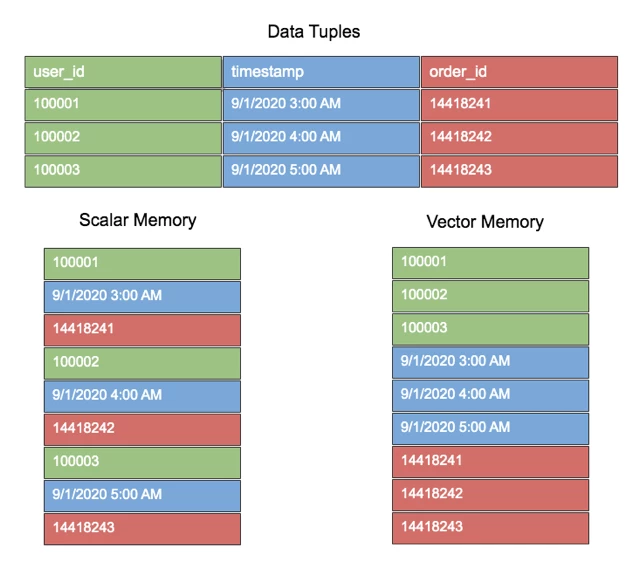
Default in-memory processing of data is row-oriented. By doing so we lose optimization opportunities if the in-memory representation is row-oriented (scalar). There are benefits of organizing data in a vector form in memory. Query execution systems typically process data one row at a time. This is intuitive for humans but not for modern CPUs, which like to process the same instructions on different data (SIMD).

Vectorization is the method or process of organizing data in memory in chunks (vector) and operating on blocks of values at a time. Figure 5 is an illustration of how a typical set of data tuples would look like in memory with scalar vs. vector memory alignment.

Figure 5: Vectorized Layout in Memory

Potential benefits of Vectorization are:

• Improved LRU CPU-cache hit ratio: When the Operating System fetches pages into the LRU cache, the CPU execution benefits from having the next instruction’s data already in the cache.
• Spark’s optimizer can create custom code to handle query operators at runtime (Whole-stage Code Generation).
• If a standard in-memory format like Apache Arrow is used to represent vector memory, it can be used for data interchange across languages bindings like Java, Python, and Javascript. This can do the following:

1. Evaluate multiple operator expressions in a single physical planning step for a batch of column values.
2. Automatic Loop Unrolling.
3. Amortize Virtual function calls: Each next() call in the batched iterator would fetch a chunk of tuples hence reducing the overall number of calls to the iterator.

Teaching Iceberg to do Vectorized Reads

Challenges

Given our complex schema structure, we need vectorization to not just work for standard types but for all columns. Our schema includes deeply nested maps, structs, and even hybrid nested structures such as a map of arrays, etc. There were multiple challenges with this. Firstly, Spark needs to pass down the relevant query pruning and filtering information down the physical plan when working with nested types. We will cover pruning and predicate pushdown in the next section.

The next challenge was that although Spark supports vectorized reading in Parquet, the default vectorization is not pluggable and is tightly coupled to Spark, unlike ORC’s vectorized reader which is built into the ORC data-format library and can be plugged into any compute framework. There is no plumbing available in Spark’s DataSourceV2 API to support Parquet vectorization out of the box. To be able to leverage Iceberg’s features the vectorized reader needs to be plugged into Spark’s DSv2 API. Since Iceberg plugs into this API it was a natural fit to implement this into Iceberg.

Vectorization in Iceberg using Apache Arrow

Apache Arrow is a standard, language-independent in-memory columnar format for running analytical operations in an efficient manner on modern hardware. It is designed to be language-agnostic and optimized towards analytical processing on modern hardware like CPUs and GPUs.

Apache Arrow supports and is interoperable across many languages such as Java, Python, C++, C#, MATLAB, and Javascript. It uses zero-copy reads when crossing language boundaries. It complements on-disk columnar formats like Parquet and ORC. For these reasons, Arrow was a good fit as the in-memory representation for Iceberg vectorization.

Iceberg is a library that works across compute frameworks like Spark, MapReduce, and Presto so it needed to build vectorization in a way that is reusable across compute engines. Iceberg now supports an Arrow-based Reader and can work on Parquet data. This implementation adds an arrow-module that can be reused by other compute engines supported in Iceberg. Adobe worked with the Apache Iceberg community to kickstart this effort. Today the Arrow-based Iceberg reader supports all native data types with a performance that is equal to or better than the default Parquet vectorized reader. Support for nested & complex data types is yet to be added.

You can track progress on this here: https://github.com/apache/iceberg/milestone/2. We intend to work with the community to build the remaining features in the Iceberg reading.

Vectorization using Native Parquet Reader

While an Arrow-based reader is ideal, it requires multiple engineering-months of effort to achieve full feature support. Adobe needed to bridge the gap between Spark’s native Parquet vectorized reader and Iceberg reading. The native Parquet reader in Spark is in the V1 Datasource API. Therefore, we added an adapted custom DataSourceV2 reader in Iceberg to redirect the reading to re-use the native Parquet reader interface. You can find the code for this here: https://github.com/prodeezy/incubator-iceberg/tree/v1-vectorized-reader. We adapted this flow to use Adobe’s Spark vendor, Databricks’ Spark custom reader, which has custom optimizations like a custom IO Cache to speed up Parquet reading, vectorization for nested columns (maps, structs, and hybrid structures).

Having said that, word of caution on using the adapted reader, there are issues with this approach. This reader, although bridges the performance gap, does not comply with Iceberg’s core reader APIs which handle schema evolution guarantees. This is why we want to eventually move to the Arrow-based reader in Iceberg.

Nested Schema Pruning and Predicate Pushdowns

As mentioned earlier, Adobe schema is highly nested. It is able to efficiently prune and filter based on nested structures (e.g. map and struct) and has been critical for query performance at Adobe. Iceberg collects metrics for all nested fields so there wasn’t a way for us to filter based on such fields.

There were challenges with doing so. In the version of Spark (2.4.x) we are on, there isn’t support to push down predicates for nested fields Jira: SPARK-25558 (this was later added in Spark 3.0). E.g. scan query

scala> spark.sql("select * from iceberg_people_nestedfield_metrocs where location.lat = 101.123".show()

In the above query, Spark would pass the entire struct “location” to Iceberg which would try to filter based on the entire struct. This has performance implications if the struct is very large and dense, which can very well be in our use cases. To fix this we added a Spark strategy plugin that would push the projection & filter down to Iceberg Data Source.

In the above query, Spark would pass the entire struct “location” to Iceberg which would try to filter based on the entire struct. This has performance implications if the struct is very large and dense, which can very well be in our use cases. To fix this we added a Spark strategy plugin that would push the projection & filter down to Iceberg Data Source.

sparkSession.experimental.extraStrategies =

sparkSession.experimental.extraStrategies :+

DataSourceV2StrategyWithAdobeFilteringAndPruning

Next, even with Spark pushing down the filter, Iceberg needed to be modified to use pushed down filter and prune files returned up the physical plan, illustrated here: Iceberg Issue#122. We contributed this fix to Iceberg Community to be able to handle Struct filtering<. After the changes, the physical plan would look like this:

// Struct filter pushed down by Spark to Iceberg Scan
scala> spark.sql("select * from iceberg_people_nestedfield_metrics where location.lat = 101.123").explain()
== Physical Plan ==
*(1) Project [age#0, name#1, friends#2, location#3]
+- *(1) Filter (isnotnull(location#3) && (location#3.lat = 101.123))
+- *(1) ScanV2 iceberg[age#0, name#1, friends#2, location#3] (Filters: [isnotnull(location#3), (location#3.lat = 101.123)], Options: [path=iceberg-people-nestedfield-metrics,paths=[]])

This optimization reduced the size of data passed from the file to the Spark driver up the query processing pipeline.

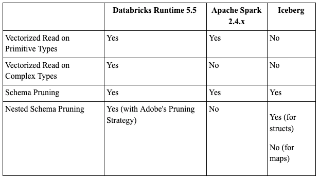
Here is a compatibility matrix of read features supported across Parquet readers.

Manifest Rewrite

As mentioned in the earlier sections, manifests are a key component in Iceberg metadata. It controls how the reading operations understand the task at hand when analyzing the dataset. Iceberg query task planning performance is dictated by how much manifest metadata is being processed at query runtime. Each Manifest file can be looked at as a metadata partition that holds metadata for a subset of data. As any partitioning scheme dictates, Manifests ought to be organized in ways that suit your query pattern.

In our case, most raw datasets on data lake are time-series based that are partitioned by the date the data is meant to represent. Most reading on such datasets varies by time windows, e.g. query last week’s data, last month’s, between start/end dates, etc. With such a query pattern one would expect to touch metadata that is proportional to the time-window being queried. If one week of data is being queried we don’t want all manifests in the datasets to be touched.

At ingest time we get data that may contain lots of partitions in a single delta of data. Iceberg writing does a decent job during commit time at trying to keep manifests from growing out of hand but regrouping and rewriting manifests at runtime. This can be controlled using Iceberg Table properties like commit.manifest.target-size-bytes. Even then over time manifests can get bloated and skewed in size causing unpredictable query planning latencies. We found that for our query pattern we needed to organize manifests that align nicely with our data partitioning and keep the very little variance in the size across manifests. In the worst case, we started seeing 800–900 manifests accumulate in some of our tables. We needed to limit our query planning on these manifests to under 10–20 seconds.

We achieve this using the Manifest Rewrite API in Iceberg. We built additional tooling around this to detect, trigger, and orchestrate the manifest rewrite operation. As a result, our partitions now align with manifest files and query planning remains mostly under 20 seconds for queries with a reasonable time-window.

While this approach works for queries with finite time windows, there is an open problem of being able to perform fast query planning on full table scans on our large tables with multiple years worth of data that have thousands of partitions. We are looking at some approaches like:

• Performing Iceberg query planning in a Spark compute job: https://github.com/apache/iceberg/issues/1422
• Query planning using a secondary index (e.g. Bloom Filters) to quickly get to the exact list of files

Before Manifest Tooling

Manifests are a key part of Iceberg metadata health. Particularly from a read performance standpoint. We have identified that Iceberg query planning gets adversely affected when the distribution of dataset partitions across manifests gets skewed or overtly scattered.

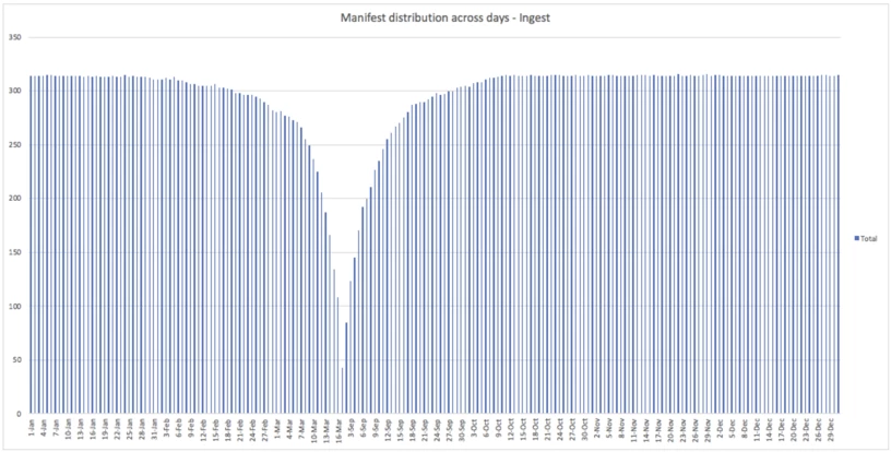
A key metric is to keep track of the count of manifests per partition. We observe the min, max, average, median, stdev, 60-percentile, 90-percentile, 99-percentile metrics of this count. The health of the dataset would be tracked based on how many partitions cross a pre-configured threshold of acceptable value of these metrics. The trigger for manifest rewrite can express the severity of the unhealthiness based on these metrics. The chart below is the distribution of manifest files across partitions in a time partitioned dataset after data is ingested over time. This illustrates how many manifest files a query would need to scan depending on the partition filter.

Figure 6: Distribution of Manifest Across Day Partitions

Iceberg Manifest Rewrite Operation

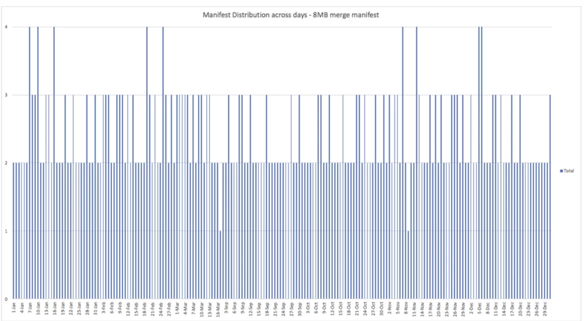
Iceberg allows rewriting manifests and committing it to the table as any other data commit. We rewrote the manifests by shuffling them across manifests based on a target manifest size. Here is a plot of one such rewrite with the same target manifest size of 8MB. Notice that any day partition spans a maximum of 4 manifests. Additionally, when rewriting we sort the partition entries in the manifests which co-locates the metadata in the manifests, this allows Iceberg to quickly identify which manifests have the metadata for a query. Iceberg supports rewriting manifests using the Iceberg Table API. This tool is based on Iceberg’s Rewrite Manifest Spark Action which is based on the Actions API meant for large metadata. The chart below is the manifest distribution after the tool is run.

Figure 7: Manifest Distribution After Manifest Rewrite

Snapshot Expiration

Snapshots are another entity in the Iceberg metadata that can impact metadata processing performance. As described earlier, Iceberg ensures Snapshot isolation to keep writers from messing with in-flight readers. This allows consistent reading and writing at all times without needing a lock. A side effect of such a system is that every commit in Iceberg is a new Snapshot and each new snapshot tracks all the data in the system. Every snapshot is a copy of all the metadata till that snapshot’s timestamp. It’s easy to imagine that the number of Snapshots on a table can grow very easily and quickly. These snapshots are kept as long as needed. Deleted data/metadata is also kept around as long as a Snapshot is around. Iceberg reader needs to manage snapshots to be able to do metadata operations. If left as is, it can affect query planning and even commit times. To keep the Snapshot metadata within bounds we added tooling to be able to limit the window of time for which we keep Snapshots around. We use the Snapshot Expiry API in Iceberg to achieve this.

Expire Snapshot Action

Iceberg supports expiring snapshots using the Iceberg Table API. For heavy use cases where one wants to expire very large lists of snapshots at once, Iceberg introduces the Actions API which is an interface to perform core table operations behind a Spark compute job. In particular the Expire Snapshots Action implements the snapshot expiry. This operation expires snapshots outside a time window. We run this operation every day and expire snapshots outside the 7-day window. This can be configured at the dataset level.

Benchmarks

In the previous section we covered the work done to help with read performance. In this section, we illustrate the outcome of those optimizations. We compare the initial read performance with Iceberg as it was when we started working with the community vs. where it stands today after the work done on it since.

Initial Read performance when we started Iceberg Adoption

We use a reference dataset which is an obfuscated clone of a production dataset. We converted that to Iceberg and compared it against Parquet. Benchmarking is done using 23 canonical queries that represent typical analytical read production workload.

• Row Count: 4,271,169,706
• Size of Data: 4.99 TB
• Partitions: 31

Figure 8: Initial Benchmark Comparison of Queries over Iceberg vs. Parquet

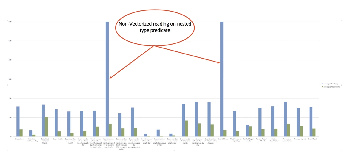
Observations

• Query Planning was not constant time. Queries with predicates having increasing time windows were taking longer (almost linear).
• We noticed much less skew in query planning times. Since Iceberg query planning does not involve touching data, growing the time window of queries did not affect planning times as they did in the Parquet dataset.
• Queries over Iceberg were 10x slower in the worst case and 4x slower on average than queries over Parquet.
• Split planning contributed some but not a lot on longer queries but were most impactful on small time-window queries when looking at narrow time windows.
• Read execution was the major difference for longer running queries.

Read Performance After Optimizations

Figure 9: Apache Iceberg vs. Parquet Benchmark Comparison After Optimizations

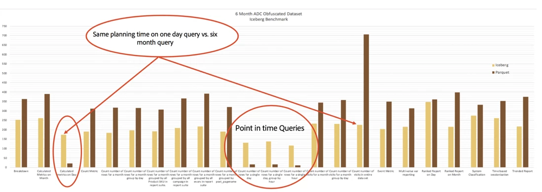
• We observed in cases where the entire dataset had to be scanned.
• Iceberg took the third amount of the time in query planning. In point in time queries like one day, it took 50% longer than Parquet. Query planning now takes near-constant time. Full table scans still take a long time in Iceberg but small to medium-sized partition predicates (e.g. 1 day vs. 6 months) queries take about the same time in planning. OTOH queries on Parquet data degraded linearly due to linearly increasing list of files to list (as expected).
• Raw Parquet data scan takes the same time or less.

Impact on Query Planning

Figure 10: Query Planning Times after Optimizations

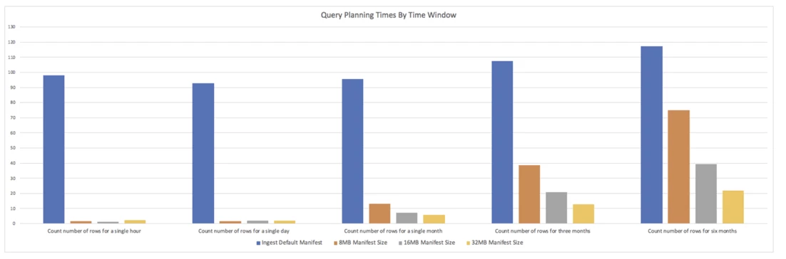
• Comparing time spent in query planning of simple count queries that span different time windows viz. 1 hour, 1 day, 1 month, 3 months, 6 months to observe impact with different manifest merge profiles.
• The default ingest leaves manifest in a skewed state. Also, almost every manifest has almost all day partitions in them which requires any query to look at almost all manifests (379 in this case).
• Repartitioning manifests sorts and organizes these into almost equal sized manifest files. So in the 8MB case for instance most manifests had 1–2 day partitions in them. So querying 1 day looked at 1 manifest, 30 days looked at 30 manifests and so on.
• Across various manifest target file sizes we see a steady improvement in query planning time. Larger time windows (e.g. 6 month query) take relatively less time in planning when partitions are grouped into fewer manifest files.

Future Work

In this article we went over the challenges we faced with reading and how Iceberg helps us with those. We illustrated where we were when we started with Iceberg adoption and where we are today with read performance. Iceberg’s design allows us to tweak performance without special downtime or maintenance windows. There are some more use cases we are looking to build using upcoming features in Iceberg. Here are a couple of them within the purview of reading use cases :

• Distributed Query Planning: In addition to the manifest metadata optimizations there are use cases where we cannot avoid a full table metadata scan e.g. GDPR actions, queries with predicates not involving a partition column (only sort key). In such events we need an efficient way to scan all metadata often for very large tables. This Iceberg github issue tracks the feature.
• Secondary Indexes: All Iceberg stats today are at the file level and can be rolled up to the partition or table level. But statistics that cannot be rolled up and are expensive to calculate, such as distinct values are useful for efficient join planning. We are working with the community on designing and building secondary indexes at the partition and table scope.
• Statistics Collection: We are building a statistical store for all our datasets to enable use cases like Cost-Based Optimization, Query Speedup on SQL queries, data quality checks. We intend to use at-rest Iceberg statistics to limit cost on such metadata collection.
• Incremental Reading: Reading deltas of appends, deletes, and update operations is a major upcoming use case for us. Furthermore, many of our internal platform customers require the ability to read updates to a dataset as a consumable stream of changes (Change Data Capture). We intend to leverage existing time travel, Copy-on-Write features, and build on the row-level delete work in the community.

In conclusion, it’s been quite the journey moving to Apache Iceberg and yet there is much work to be done. We look forward to our continued engagement with the larger Apache Open Source community to help with these and more upcoming features.

Follow the Adobe Experience Platform Community Blog for more developer stories and resources, and check out Adobe Developers on Twitter for the latest news and developer products. Sign up here for future Adobe Experience Platform Meetups.

Related Blogs

• Iceberg at Adobe
• High Throughput Ingestion with Iceberg

References

1. Adobe Experience Platform
2. Apache Iceberg
3. Distributed Job Planning #1422
4. Apache Spark Table API
5. Loop unrolling
6. Apache Iceberg Vectorized Read
7. Apache Iceberg V1 Vectorized Reader
8. SPARK-25558
9. Iceberg Issue#122
10. Apache Iceberg Manifest Rewrite API
11. Apache Iceberg Snapshot API
12. Apache Iceberg time travel
13. Apache Iceberg Copy-on-Write
14. Apache Iceberg Row-Level-Delete-Work

Originally published: Jan 14, 2021