How Adobe Does Millions of Records per Second Using Apache Spark Optimizations – Part 2

[#1]

Authors: Yeshwanth Vijayakumar, Vineet Sharma, and Sandeep Nawathe

In Part 1, we went over how we applied some Spark optimizations to our Structured Streaming Workloads. In Part 2, this blog details how we optimized our Interactive Query Evaluation workloads on top of Apache Spark. This blog post is adapted from this Spark Summit 2020 Talk.

Architecture Overview

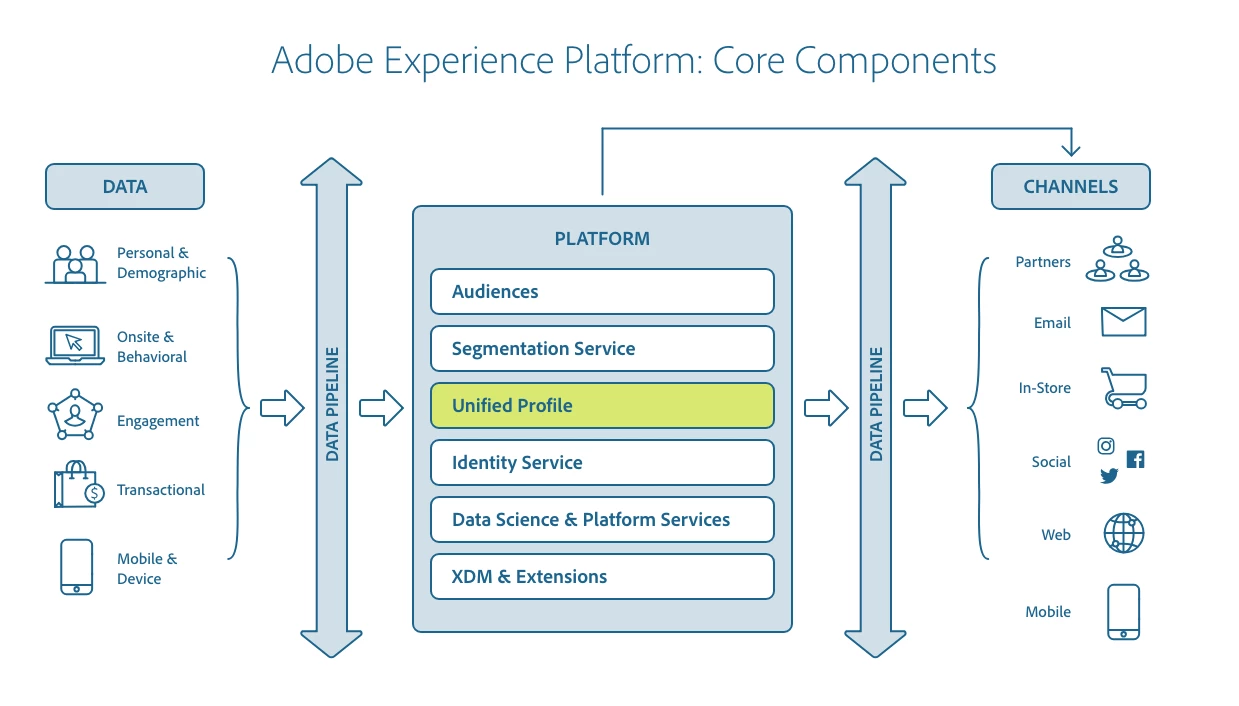
Just as a reference from the previous blog to set the context. Here again is the relationship between Adobe Experience Platform Real-time Customer Profile and other services within Adobe Experience Platform is highlighted in the following diagram:

Figure 1: High-level architecture

Our Requirements

Adobe Experience Platform assimilates data from various channels and makes this data actionable for targeting and marketing experiences. Our customers needed to express their segments as rules to the platform and it takes care of executing these complex rules in a high performant fashion. Therefore, our requirements were at a high level:

• Build an interactive segmentation which offers real-time responsive results on the subset of the merged profile data.
• Build an interactive component to begin getting results and feedback as a result of the query right from the time a query begins evaluation instead of waiting till the end of execution to get the results.
• Build a component that uses a long-running Spark application that accepts queries and executes them using the PQL execution engine — PQL Overview.

Evaluation Optimizations

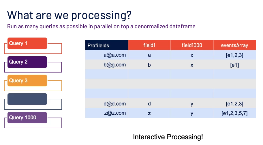
The figure below shows the context of the processing, wherein we have pre-computed a merged view of customer profiles across various identities (email IDs, CRMID, and ECID) and sources (Adobe Analytics, CRM, and Custom). We then take thousands of segmentation rules defined in Profile Query Language and execute them concurrently in one shot. Our throughput is defined by how many profiles and records are we able to segment.

Given that we are running multiple new queries interactively on top of the same snapshot of data, the read IO is constant and optimized by caching/persisting the dataframe. The measure of how well we are doing is decided by achieving a higher throughput of records processed and the interactivity component by how quickly we start returning/processing results back to the user once a query is submitted.

Figure 2: Overview of the processing landscape

The Art of Caching My Physical Plans

In the case of Interactive Query Processing, we can visualize the problem as executing the same function runQuery (queries=[q1,q2..]) on top of the same data frame for different query inputs.

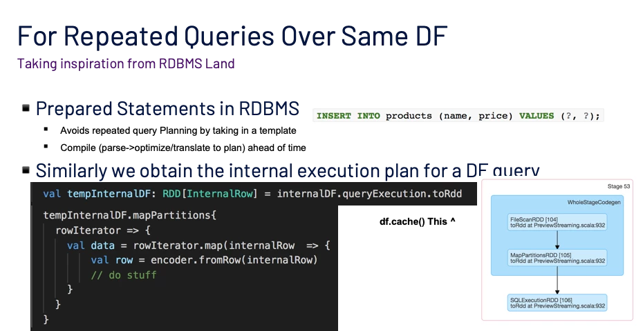
Given that it is the same unit of work being run on the underlying data, we should utilize this notion in our optimization. We will take some inspiration from the preparedStatements in RDBMS.

Figure 3: Introduction of the Repeated Query Use-case

Let’s take a look at which bottleneck we are trying to overcome. We look at it through the lens of an interactive query processing perspective here latency of returned results plays an important role.

The Spark dataframe has 1000’s of simple or nested columns. For example, simple columns like churnScore or nested fields like person.gender, `optInOut, or channels.directMail. Just printing the Spark query plan causes an overflow while printing to logs in debug mode. The time for query planning takes more than 2–3 seconds on average and in some worst cases up to 7 seconds. This makes a significant impact while submitting interactive queries when the total runtime of the query is less than 10s end to end from the time of query submission.

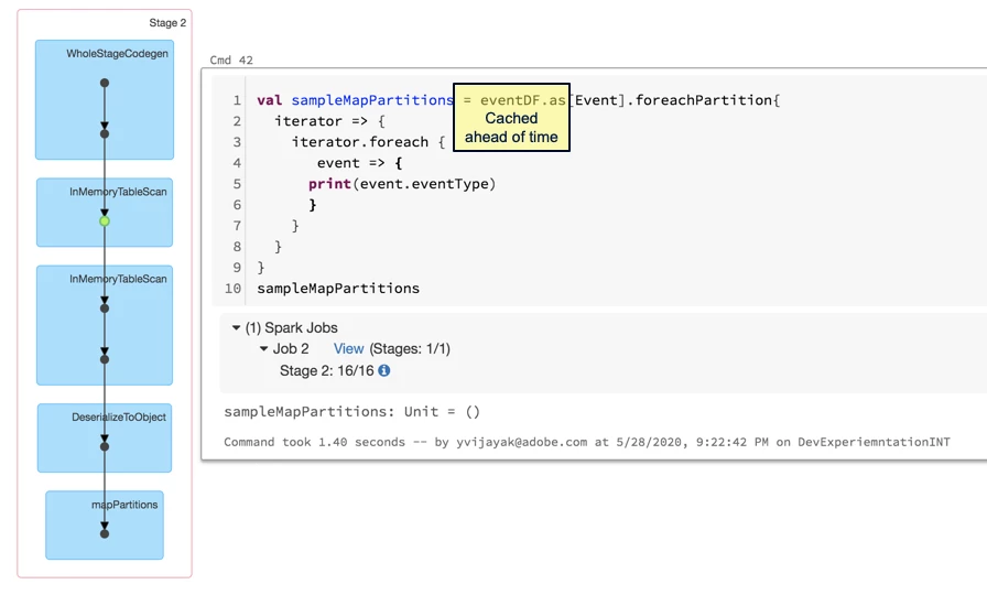
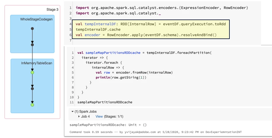
Figure 4 shows a barebones version of our query evaluation scenario, we replace the actual query processing logic with a println to simulate an IO operation. We use this example to not pollute our experiment with the actual evaluation logic and to focus on the surrounding harness.

The eventDF is the data frame containing the list of events we are going to run the scenario over. We cache the data frame ahead of time using eventDF.persist (StorageLevel.MEMORY_ONLY) to make sure we get the best performance possible. Even with data caching the planning step is still repeated every time the query/job is executed, thus while we are good on the read/evaluation throughput, we still are bottlenecked by repeated planning.

Figure 4: Before: Physical Plan Caching, with only dataframe caching

The dataframe.queryExecution.toRDD returns the Spark Physical plan which is the downstream step after the Analyze and Planning Step. We intend to hijack this step and reuse it.

Inspiration was from this Stack Overflow Answer.

This step returns an RDD[InternalRow] hence we need to apply the row transformation to each row, which is quite cheap since it’s a sparse row but skips the planning stage which is expensive due to the size of the metadata(> 1000 nested columns).

Figure 5: After- Physical Plan Caching, query execution time dropping to less than half of the previous time

Know Thy Join

Join Optimization For Interactive Queries (Heavily Opinionated)

Since the Adobe Experience Platform Real-Time customer Profile ingests data from various sources, which could involve non-entity data such as for example product catalogs and offer inventory. We needed to do a real-time join with these non-person entities to create even more sophisticated segmentation queries. Having an interactive query experience and joins at the same is not exactly convenient. We go over a few recommendations:

• Avoid them by de-normalizing if possible. If you are able to have a denormalized structure that would be the best case. Though you would have to deal with update amplifications in the worst case.
• Broadcast the Join Table if it’s small enough. You can simulate a HashJoin in the RDBMS world. This way you make good use of the memory in your Spark cluster.
• If too big to broadcast, check if the join info can be replicated into Redis like KV Stores. You still get the characteristics of Hash Join. This gets around the memory constraint by offloading it to a network-oriented load for lookups.
• Once you get into really large data, Shuffles will hate you and vice versa! Sort-Merge Join is your friend until it isn’t, given an interactive use-case it’s a non-starter. Shuffle Read/Write performance from disk will definitely work against real-time results, though you can always throw some money in the form of SSD for it.

Skew! Phew!

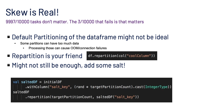
Data skewness is a problem that usually surfaces once you get your application out into the real world. Given the dynamic nature of it, just throwing more resources at it might not be an ideal solution. In Spark, it does not matter that 9999/10000 of your tasks succeed, the 1/10000 that failed will block the progress of your job and eventually fail it.

Figure 6: A salty proposal for skewness

How to get the magic targetPartitionCount?

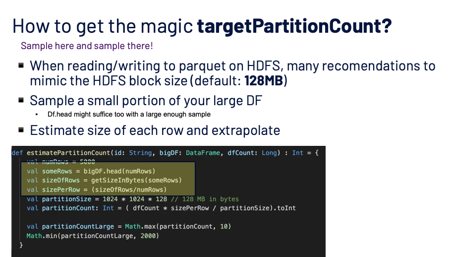
Sample here and sample there! That’s the biggest and cheapest tip that will get us out of this conundrum. Figure 7 below explains how to go about doing it.

Figure 7: Guidance for partition count inference

Putting Everything Together

Figure 8: Comparison of the interactive jobs before and after applying the techniques

Special Mention: Redis — The Ultimate Swiss Army Knife

We utilize Redis as an intermediate store for a lot of the counters/data being emitted from the Spark Jobs and it fits the bill since it’s a high-performance data structure store. Redis is an in-memory data store with some optional persistence options and can handle thousands of requests per second easily even with minimum configurations. Having a JVM local cache adds a lot of memory pressure, by storing the cached data structures off-heap, we are no longer limited by JVM memory but offload it to more network bandwidth since it means more round trip calls to Redis.

Using Redis With Spark Uncommonly (Depends on whom you ask)

• Maintain Bloom Filters/HLL on Redis. Since Redis is a data structure store, we can use the inbuilt bit vector-based operations to keep track of probabilistic data structures.
• Interactive Counting while processing results using mapPartitions. Spark Accumulators are error-prone and slow. We can replace them with Redis hashes and counters.
• Event Queue to Convert any normal batch Spark to Interactive Spark. It's not necessary to add Apache Kafka as a queuing layer for every application. Using Redis Queues, we can easily implement simple or priority-based work/execution queues on the Spark Driver and spawn queries accordingly.

Best Practices

• Use Pipelining + Batching: We go deeper into Pipelining in the next section.
• Tear down connections diligently: Having zombie connections adds to the memory pressure as well as erroneous operations when switching context.
• Turn off Speculative Execution: Speculative Execution assumes that duplicate tasks’ results/side effects can be consistently resolved. If not we can end up with double counting. If you do want to use Speculative Execution, you might want to have extra data structures to do bookkeeping from a partition level.

Digging into Redis Pipelining + Spark

How we publish data to Redis from the tasks in the executor has a big difference in the throughput of the job.

Let’s look at pipelining here in the figure below. To quote the Redis documentation:

A Request/Response server can be implemented so that it is able to process new requests even if the client didn’t already read the old responses. This way it is possible to send multiple commands to the server without waiting for the replies at all, and finally read the replies in a single step.

Figure 9: Pipelining vs no pipelining

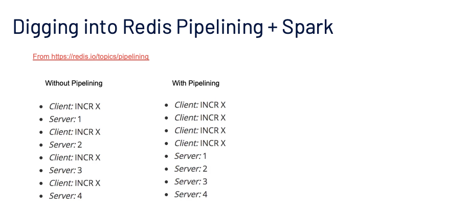
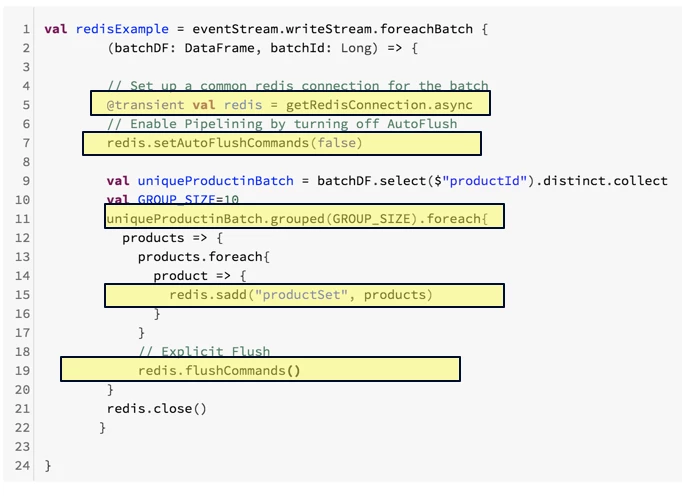
This means we are effectively able to micro-batch sending commands to Redis without having to actually wait for an ACK. This is a very important property in the case of mapPartitions since we are iterating through a partition in a linear fashion, we can group together multiple changes before issuing a blocking wait for an ack from Redis. That way Redis handles the queuing on the server-side. In the example below, we can see how we use the grouped(BATCH_SIZE) operator to effectively batch together changes for a group of rows before sending it to Redis.

There are some caveats. If your task has any operations that need to operate within a Redis Transaction, pipelining might not be a good fit. Depending on the client library used, you will need to tune the Command Queue size (for example lettuce-core, the client.requestQueueSize controls the queue size). Make sure to benchmark the GC and OOM while using pipelining, since the requests are buffered on the client-side:

• Look into enabling off-heap storage if your client uses netty -D=io.netty.noPreferDirect=true

Figure 10: Example of Redis pipelining within a Spark foreachBatch

Conclusion

In conclusion, we have presented multiple Spark optimizations over the Structured Streaming Statistics pipeline and the interactive query processing use cases. These learning have helped tremendously in our scaling process as we keep adding more value to our customers. We look forward to presenting more optimizations in other areas of distributed computing that we apply in the Adobe Experience Platform. We hope what we have shared in these blog posts is useful in any way to your adventures with Apache Spark.

Follow the Adobe Experience Platform Community Blog for more developer stories and resources, and check out Adobe Developers on Twitter for the latest news and developer products. Sign up here for future Adobe Experience Platform Meetups.

References

1. Overview — Adobe Experience Platform Real-time Customer Profile
2. Documentation —Adobe Experience Platform Real-time Customer Profile
3. Apache Spark
4. Databricks
5. Profile Query Language
6. Burrow
7. Lettuce-core
8. Redis

Originally published: Nov 19, 2020