How Adobe Does Millions of Records per Second Using Apache Spark Optimizations — Part 1

[#1]

Authors: Yeshwanth Vijayakumar, Vineet Sharma, and Sandeep Nawathe

Adobe Experience Platform enables you to drive coordinated, consistent, and relevant experiences for your customers no matter where or when they interact with your brand. With Adobe Experience Platform Real-time Customer Profile, you can see a holistic view of each individual customer that combines data from multiple channels, including online, offline, CRM, and third party data. It allows you to consolidate your disparate customer data into a unified view offering an actionable, timestamped account of every customer interaction.

In this blog post, we will describe our optimization techniques done to scale our throughput using Apache Spark. In particular, we will describe two stages of Unified Profile Processing where we use Apache Spark heavily and discuss techniques we have learned during optimizing these. This blog post is adapted from this Spark Summit 2020 Talk.

Architecture Overview

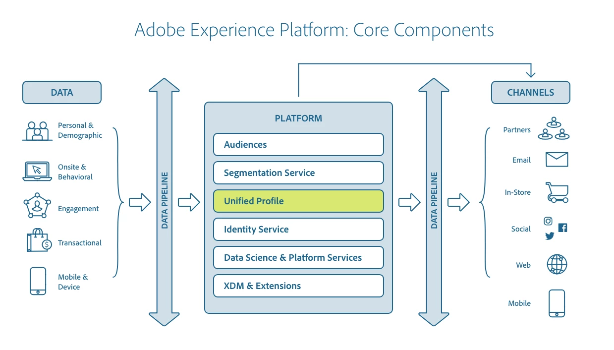
Given that the Adobe Experience Platform assimilates data from various sources, Real-time Customer Profile acts as the central hub ingesting data from different data sources; it stitches data together with the Adobe Identity Service and ships the data to various marketing destinations to enable new experiences.

The relationship between Adobe Experience Platform Real-time Customer Profile and other services within Adobe Experience Platform is highlighted in the following diagram:

Figure 1: High-level architecture

Focus Area: Post Ingestion Stats Generation

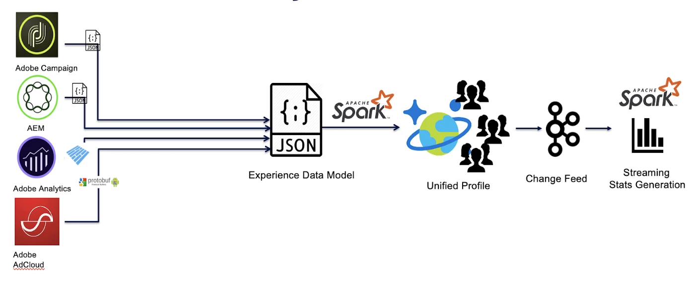
When data is ingested into Profile from various sources, each mutation to the profile store generates a change feed message sent on a Kafka Topic. This firehose is consumed by a Spark Streaming Application to generate various statistics on top of the data in real-time. We have a need to generate streaming statistics such as data-source based metrics and real-time aggregates on top of the Adobe Experience Platform Real-time Customer Profile. These computations are used by various internal services for operations like segmentation and data export.

Figure 2: Ingestion Workflow for Adobe Experience Platform’s Unified ProfileLet’s dig into what we did to get the maximum juice out of Spark.

Streaming Optimization Techniques

Know Thy Lag — How to measure

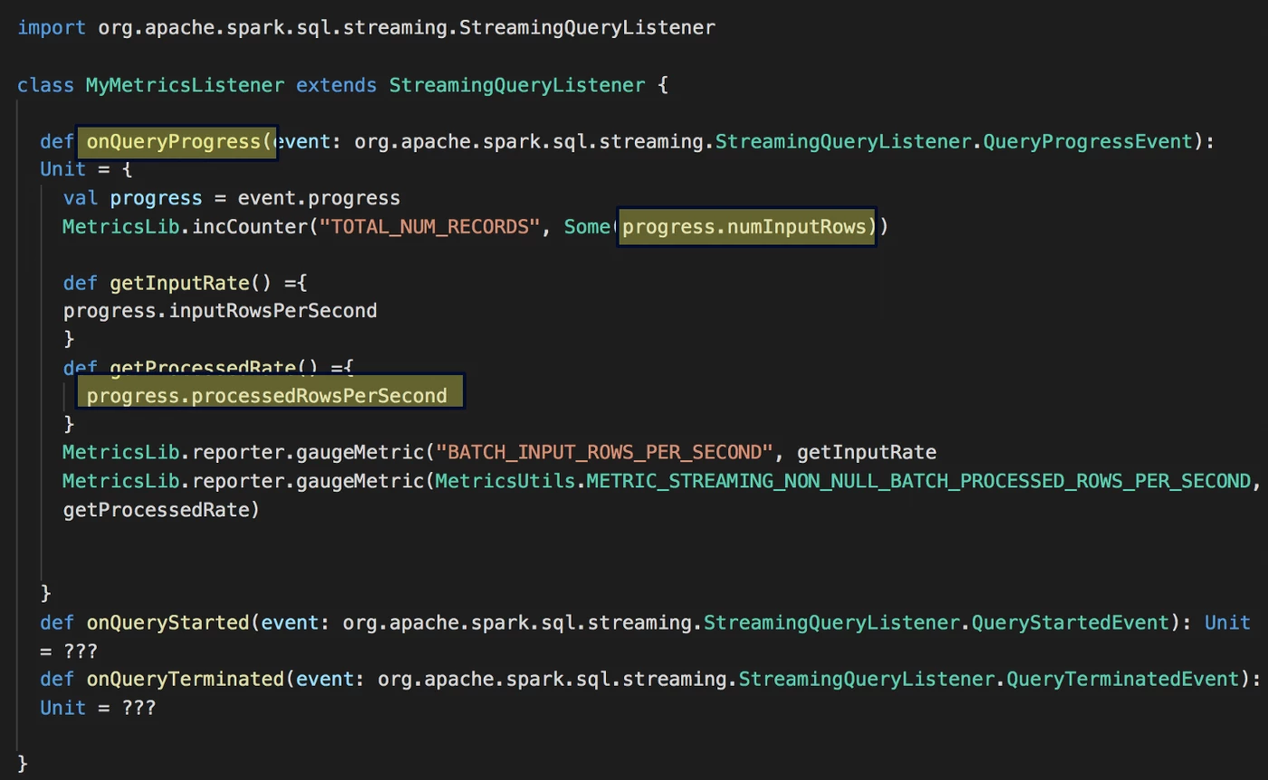
Having a streaming-based ingestion mechanism makes it that much harder to track. We will specifically use the StreamingQueryListener to keep track of the progress as we consume from Kafka

At the minimum, in order to track the progress, we will hook into the QueryProgressEvent which exposes a lot of in-depth metrics like (but not limited to):

• Duration details and statistics: Time is taken by the microbatch for processing batchDuration and Max/Min/Watermark event timestamps related to the micro-batch.
• numInputRows: Aggregate (across all sources) number of records processed in a trigger.
• processedRowsPerSecond: Aggregate (across all sources) rate at which Spark is processing data
• SourceProgress: Information about the offsets of the topic(s) the current micro-batch has processed.

Figure 3: Example of Custom StreamingQueryListener to update custom metrics

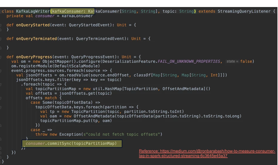
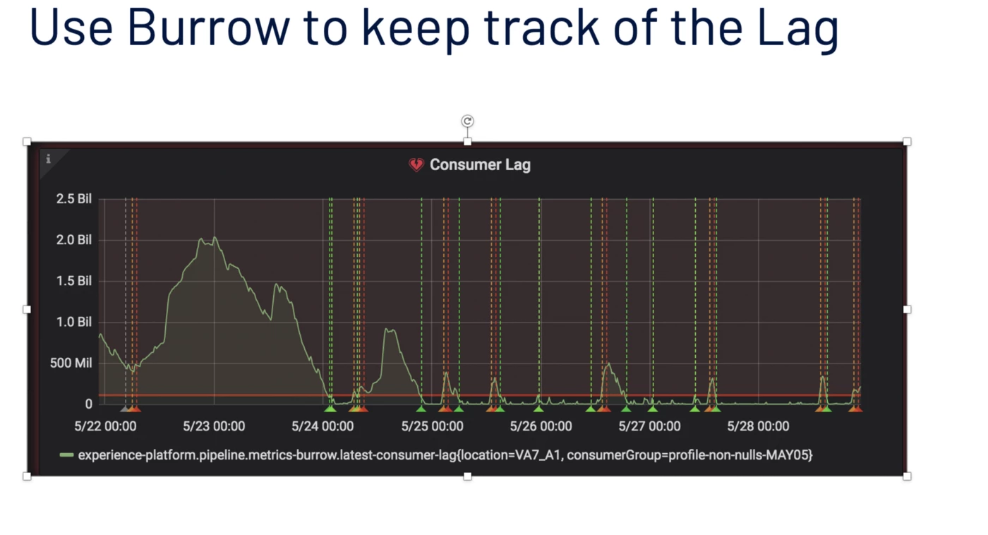
We also need to keep track of how much progress we have made in the Kafka topic relative to the latest offset. Burrow is a monitoring companion for Apache Kafka that provides consumer lag checking as a service without the need for specifying thresholds. It monitors committed offsets for all consumers and calculates the status of those consumers on demand.

We create a Dummy Consumer group in Kafka for a topic and commit the offsets of progress as extracted from the EventProgress object.

There is an aspect of convolution to take into account because Spark structured streaming automatically creates a consumer group to track the progress per query but it is not possible to deterministically retrieve it. The code shows that each query instance generates a unique Kafka Consumer Group id and currently it is not possible to explicitly assign a group.id as per v2.4.0.

Figure 4: Custom SparkQueryListener to keep track of Kafka topic lag in a Dummy ConsumerGroup

Figure 5: Example of visualizing lag from Burrow and displaying it on Grafana

Structured Streaming Specific Optimizations

We are going to explore multiple aspects of optimizing our streaming statistics pipeline by looking at how to optimize reading data from the Kafka firehose. Then we will move onto setting some best practices for expressing the logic. Lastly, we will touch base on Speculative Execution which will help with stability and performance guarantees.

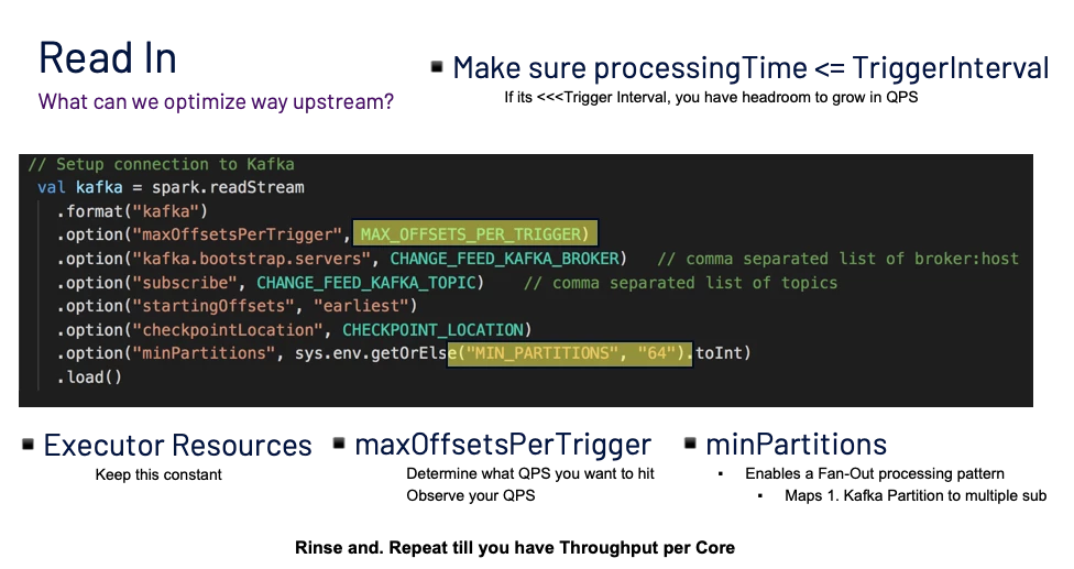
Read-in Data from Kafka Topic — Optimize the Upstream

A good amount of performance bottlenecks can exist when we are reading from the Kafka Topic, hence in order to get our desired throughput, it makes sense to focus on what we can tune to get maximum read performance.

Let’s take a look at some parameters that we feed into the Kafka spark source that we tuned and led to a throughput increase:

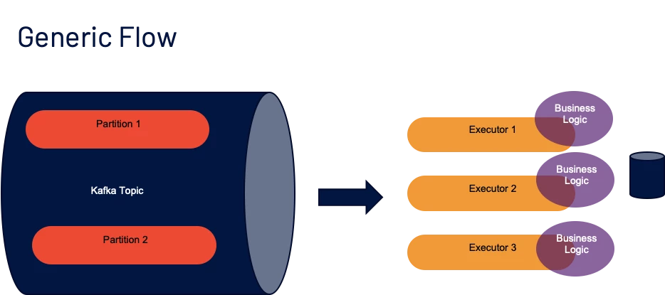
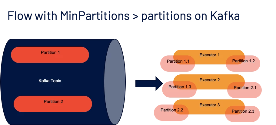
• minPartitions — The desired minimum number of partitions to read from Kafka.

** By default, Spark has a 1–1 mapping of topicPartitions to Spark partitions consuming from Kafka.

** If we set this option to a value greater than our number of topicPartitions, Spark will map the input Kafka partitions to subpartitions on the Executor side. I.e if you have 6 partitions on your Kafka Topic, but you set minPartitions to 12, roughly, each input partition might be mapped to 2 subpartitions on the Spark side.

** This is by far the biggest performance enhancer, since often as a consumer we do not have control over the number of partitions of the topic(s) we consume from.

** Also, there is a good chance the Spark Job has access to more cores than there are input partitions, in that case having a 1–1 mapping wastes resources that are already allocated, hence specifying a good value here makes a great difference in good read throughput

• maxOffsetsPerTrigger — Limits the maximum number of offsets that are pulled from Kafka.

** The specified total number of offsets will be proportionally split across topicPartitions of different volumes.

** This is a replacement for backpressure since we control how much to pull based on what load we can process.

Figure 7: Generic dataflow from a Kafka topic to Spark Executors

Figure 8: Mapping of Kafka partition to subpartitions in the executors enabling Fan-Out consumption pattern

We experimented with the following two metrics and Figure 9 explaining the results:

• Trigger Interval — At what frequency a micro-batch will be triggered
• Processing Time — Time that is taken for processing by the micro-batch

Figure 9: Read Optimizations Experiment Cycle

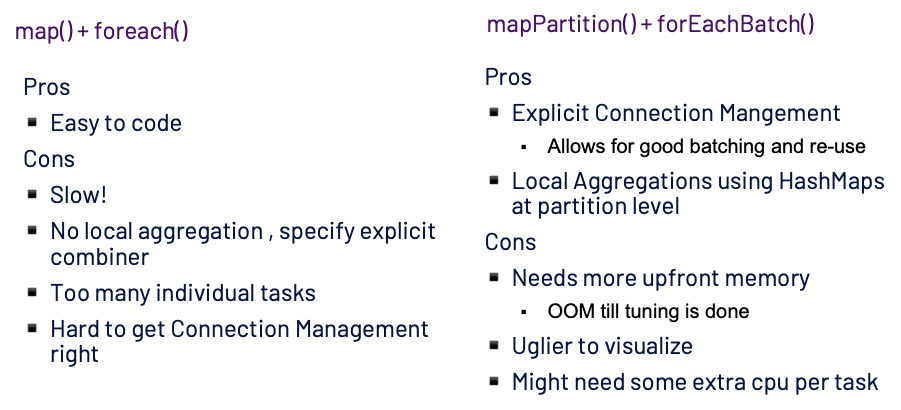
MicroBatch Hard! — Best Practices

When we micro-batch, we are presented with two options to express our business logic, using a map + foreach or a mapPartitions partition. There is no right or wrong way, though understanding the trade-offs as presented below can save you a good amount of time instead of sitting with a profiler tool.

Figure 10: Overview of map()+ foreach() Vs mapPartition() + forEachBatch()

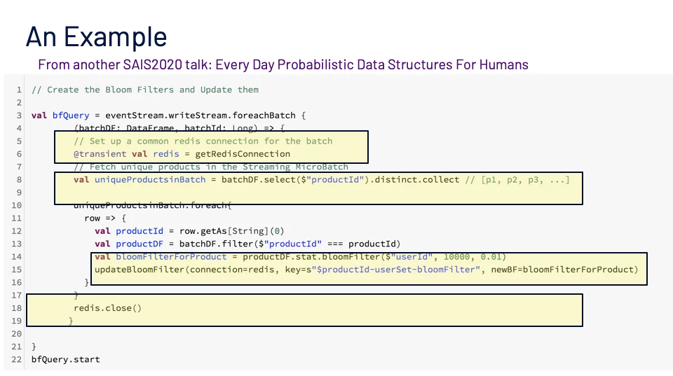
Tip: spark.task.cpus controls how many cores you want to allocate per task, usually neglected, but if you are switching to a foreachBatch type workload, you might want to bump it up since it has an indirect effect of increasing memory per task.

Figure 11 shows an example use of foreachBatch. This example shows the use of a top-level Redis Connection redis to be shared by the task components. The calculation of the uniqueProductInBatch attribute shows pre-processing and aggregating data locally at the task level for a partition. We see an example of utilizing the common top-level connection in the usage of the updateBloomFilter() function. An explicit teardown of top-level- shared connection is shown at the end of the foreachBatch with a redis.close().

Figure 11: Example showing efficient use of foreachBatch

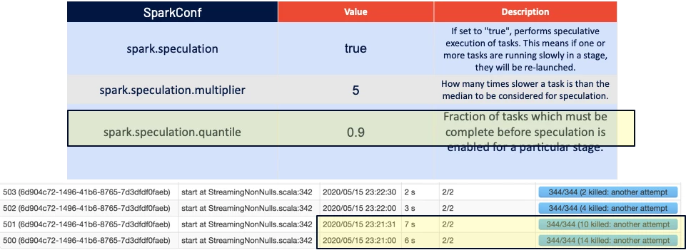
Speculate Away!

Sometimes even if all other aspects of your application is tuned, you could run into some rough times due to:

• Traffic spikes
• Uneven distributions in data in partitions leading to GC pauses
• Noisy neighbors for tasks within an executor
• Virtual machine issues leading to bad executor performance

To get around this Spark has an inbuilt mechanism to keep an eye on the task times and their distributions. If Speculative Execution is enabled, Spark will monitor the tasks and if it notices a bunch of them running slowly it will start new instances of it and will kill the slow running ones.

This maintains the average run times of the micro-batches to an extent so that you do get hung jobs.

Tip: The spark.speculation.multiplier and spark.speculation.quantiile give granular control on the details of the speculation.

Note that even if a single task for your micro-batch does not complete, the next micro-batch cannot start. This tip is not just for performance reasons, but also for making sure the functional aspect of your application is reliable.

Figure 12: Example showing Spark Speculation proactively killing slow tasks to keep average runtime in control

Here are some caveats for Speculative Execution. Your task’s side effects need to account for duplicate tasks being spawned off. For example, if you have a side-effect of incrementing a counter on Redis, your incrementing logic needs to be partition/task-aware. Otherwise, you will end up double counting. This won’t help in the case of data-skewness, since no matter how many times you run a skewed task if it exceeds the max resources you have, it's a no-go (We tackle this problem including how we optimized our evaluation processing with Spark pipelines in my next blog post).

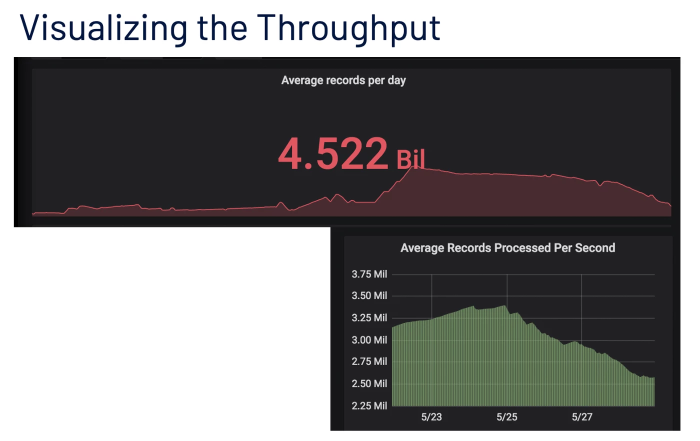
Conclusion and Putting Everything Together

The techniques described above helped us scale our post-ingestion streaming pipeline and we were able to achieve consistent peak throughputs exceeding a million records a second consistently with no manual intervention during heavy traffic peaks. As the following figure indicates, currently we process around 4 billion messages a day with multiple peaks in the day. We also show the trend of the average number of records processed per second peaking around the 3.2 million mark after having incorporated the techniques discussed above.

Part 2 of this blog will detail further details of optimization and results.

Follow the Adobe Experience Platform Community Blog for more developer stories and resources, and check out Adobe Developers on Twitter for the latest news and developer products. Sign up here for future Adobe Experience Platform Meetups.

References

1. Adobe Experience Platform Unified Profile
2. Apache Spark
3. Databricks
4. Burrow
5. “How to Measure Consumer Lag in Spark Structured Streaming”, Ron Barabash
6. Redis documentation
7. Grafana

Originally published: Nov 12, 2020